| Collapse All
3.0: Input Format Requirements
3.0.1: AGP
AGP files provided with the --agp argument (see Section 3.1.2 below) must conform the NCBI’s AGP v2.0 specification. Please visit the following link for details:
3.0.2: FASTA
GAEMR relies on Biopython for most FASTA processing, so input FASTA sequences should conform to the format in the following link:
3.0.3: BAM & Read Lists
GAEMR requires a list of BAM files in CSV file format supplied to it view the --read_list (-l). The first line of the file is the header and should look like this:
#name,lib_type,mean_read_len,dir,insert_size,files
The following table describes the header items. Note that some of these options do not apply to certain library types, and therefore should be left blank within the CSV file (see example below):
[table delimiter=”|”]
Field|Description
name| The library’s identifier
lib_type| The library type (fragment, jump, unpaired)
mean_read_length| The mean read length of the reads
dir| The expected direction of paired reads with respect to each other (FR is forward and reverse, RF is reverse and forward)
insert_size| The mean insert size for the library
files| The full file path for the library’s bam file
[/table]
The following example demonstrates a read list file specifying fragment pair, jump pair, and PacBio unpaired data, in that order.
#name,lib_type,mean_read_len,dir,insert_size,files

C0DJUACXX.1.Pond-121053,fragment,101,fr,200,/my/bam/file/directory/fragments.bam

C0DJUACXX.2.Solexa-76388,jump,101,rf,3000,/my/bam/file/directory/jumps.bam

All.PacBio,unpaired,900,,,/my/bam/file/directory/long_reads.bam
Note that ‘dir’ and ‘insert_size’ are not supplied for the PacBio data because they do not apply to this read type.
3.1: GAEMR Arguments
GAEMR arguments may be specified with either a single-dashed short form argument or a double-dashed long form argument. For arguments requiring a specific value, the short form argument should be followed by a space and then the value, and the long for argument should be followed by an ‘=’ sign and the value. See the tables in section 3.1.1 and 3.1.2 below for details.
3.1.1: Required Arguments
At least one of the following arguments must be specified for GAEMR to run:
[table delimiter=”|”]
Argument|Description|Example
-s SCAFFOLDS~~--scaffolds=SCAFFOLDS|Specifies a scaffolds FASTA file to use for analysis (Default=none)|GAEMR.py -s scaffolds.FASTA
-c CONTIGS~~--contigs=CONTIGS|Specifies a contigs FASTA file to use for analysis (Default=none)|GAEMR.py -c contigs.FASTA
[/table]
3.1.2: Optional Arguments
The following arguments may be used in any combination to produce more data or to further customize the analysis run.
[table delimiter=”|” nl=”~~”]
Argument|Description|Example
-h~~--help|Prints GAEMR usage information to screen|GAEMR.py -h~~GAEMR.py --help
-r REFERENCE~~--reference=REFERENCE|Specifies the reference file to use for analysis (default=none)|GAEMR.py -r reference.FASTA~~GAEMR.py --reference=reference.FASTA
-a AGP~~--agp=AGP|Specifies an AGP file for analysis(default=none)| GAEMR.py -a genome.agp~~GAEMR.py --agp=genome.agp
-l READ_LIST_FILE~~--readlist=READ_LIST_FILE|Specifies the list of reads to use for alignment(default=none)|GAEMR.py -l reads.list~~GAEMR.py --readlist=reads.list
-t THREADS~~--threads=THREADS|Indicates the number of threads to use for multi-threadable processes(default=1)| GAEMR.py -t 4~~GAEMR.py --threads=4
-w WINDOW_SIZE~~--window_size=WINDOW_SIZE|Selects the window size for chart outputs (default=1000)|GAEMR.py -w 500~~GAEMR.py --window_size=500
-n ASSEMBLY_NAME~~--assembly_name=ASSEMBLY_NAME|Name of assembly (default=assembly)|GAEMR.py -n my_assembly~~GAEMR.py --assembly_name=my_assembly
-m ASSEMBLER~~--assembler=ASSEMBLER|Assembler used to generate consensus(default=assembler)|GAEMR.py -m allPaths~~GAEMR.py --assembler=allPaths
-o OUTPUT~~--output=OUTPUT|Output header (default=assembly)|GAEMR.py -o my_assembly~~GAEMR.py --output=my_assembly
-b BLAST_TASK~~--blast_task=BLAST_TASK|Type of blast to run for contamination check: blastn, dc-megablast, megablast (default=megablast)|GAEMR.py -b blastn~~GAEMR.py --blast_task=blastn
-i ALIGNER~~--aligner=ALIGNER|Aligner to use for reads alignments: bwa or bowtie2(default=bwa)|GAEMR.py -i bowtie2~~GAEMR.py --aligner=bowtie2
-k KMER_SIZE~~--kmer_size=KMER_SIZE|k-mer size for repeat and k-mer coverage stats (default=29)|GAEMR.py -k 100~~GAEMR.py --kmer_size=100
--no_blast|Do not run blast jobs (default=false)|GAEMR.py --no_blast
--minScaffSize=MINSCAFFSIZE|Minimum scaffolds size for inclusion in analysis(default=1)|GAEMR.py --minScaffSize=1000
--minConSize=MINCONSIZE|Minimum contig size for inclusion in analysis(default=1)|GAEMR.py --minConSize=500
--minGapSize=MINGAPSIZE|Minimum length of a string of Ns to determine a gap(default=10)|GAEMR.py --minGapSize=50
[/table]
3.2: Output Reference
The GAEMR html page provides quick access to the charts and tables produced by GAEMR for a particular assembly.
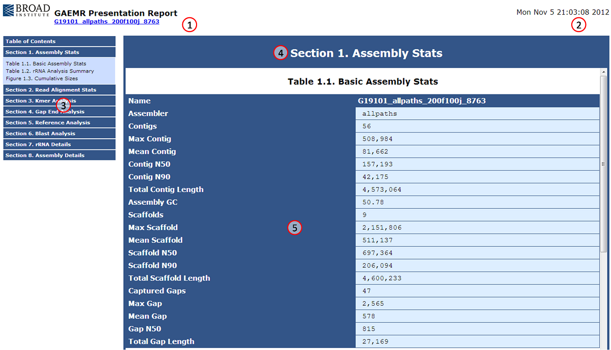
| Number|Name |Description |
|---|
| 1| Assembly Report Header| This header displays the name of the assembly that was analyzed, a link to the assembly web page, and a logo. |
| 2|Run Date| This is the date and time the analysis was executed. |
| 3|Navigation Panel| These are the eight analytical sections produced by GAEMR. Each section can be clicked on to show the individual tables and figures of the section. In this screenshot, Section 1 has been expanded to display its contents. |
| 4|Section Header|This is the header for the section last selected from the navigation panel. |
| 5|Information Panel|This is where the tables and figures for the last selected section are displayed. The bar on the right allows users to scroll to additional information within the section. |
Sections 3.2.1-3.2.8 below describe each table or figure with examples. The module that produces each table or figure is also indicated inside parenthesis beside the table or figure title.
3.2.1: Assembly Stats
Table 1.1: Basic Assembly Stats (basic_assembly_stays.py)
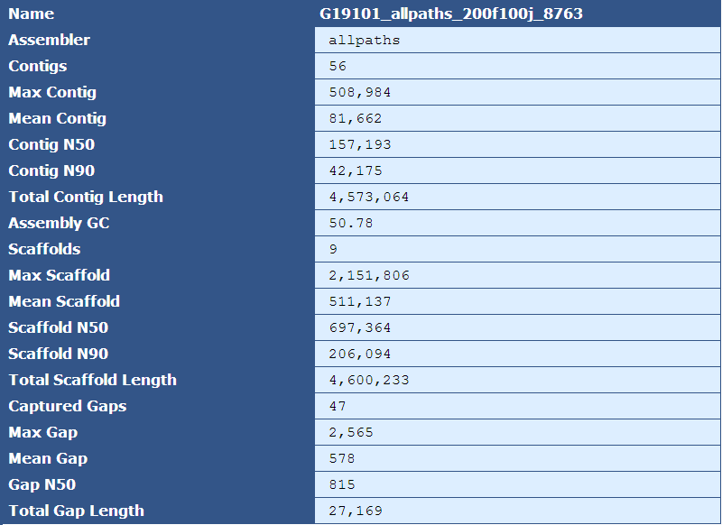
The header for this table identifies the name of the assembly, as specified by the --assembly_name (-n) option. The rows are described by the following table:
[table delimiter=”|”]
Descriptor| Description
Assembler|The assembler used for assembly, as specified by the --assembler(-m) option
Contigs|The number of contigs in the assembly
Max Contig|The length(in bases) of the largest contig in the assembly
Mean Contig|The mean size of the contigs in the assembly
Contig N50| The length of the contig in which all larger contigs in the assembly would compose 50% of the genome
Contig N90| The length of the contig in which all larger contigs in the assembly would compose 90% of the genome
Total Contig Length| The sum of the lengths of all contigs in the assembly
Assembly GC|The percent of G and C bases in the assembly
Scaffolds|The number of scaffolds in the assembly
Max Scaffold|The length of the largest scaffold in the assembly
Mean Scaffold|The mean size of the scaffolds in the assembly
Scaffold N50|The length of the scaffold in which all larger scaffolds in the assembly would compose 50% of the genome
Scaffold N90| The length of the scaffold in which all larger scaffolds in the assembly would compose 90% of the genome
Total Scaffold Length|The sum of the lengths of all scaffolds in the assembly
Captured Gaps| The number of gaps spanned by jump reads
Max Gap|The predicted size of the largest gap
Mean Gap|The predicted mean size of all the gaps
Gap N50| The size of the gap in which all larger gaps in the assembly would compose 50% of all missing sequence
Total Gap Length|The sum of the sizes of all gaps in the assembly
[/table]
Table 1.1: rRNA Analysis Summary (analyze_rna_hits.py)
This table provides results on GAEMR’s rRNA analysis module. The contents are described in the following table:
[table delimiter=”|”]
Descriptor| Description
Gene| The gene identified in the assembly
Total Copies| The number of copies of the gene in the assembly
Lineage| The lineage of the organism found
Number of Organisms Found| The number of different organisms identified by rRNA analysis
Organism IDs| The genus of the organism
[/table]
Figure 1.3: Cumulative Sizes (basic_assembly_stats.py)
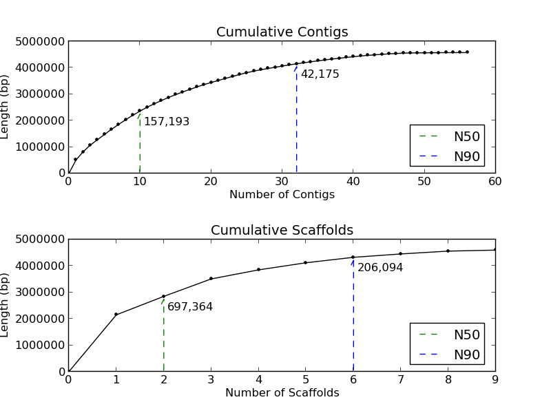
The Cumulative Sizes plots give the user an indication of how many contigs and scaffolds compose 50% and 90% of the analyzed genome. In this example, the contigs plot (top) demonstrates that 50% of this genome is in 10 contigs, and 90% in 32 contigs. The scaffold plot (bottom) shows 50% of the genome is in 2 scaffolds, and 90% of the genome is in 6 scaffolds.
3.2.2: Read Alignment Stats
Figure 2.1: Coverage Line Plot and GC (generate_bam_plots.py)
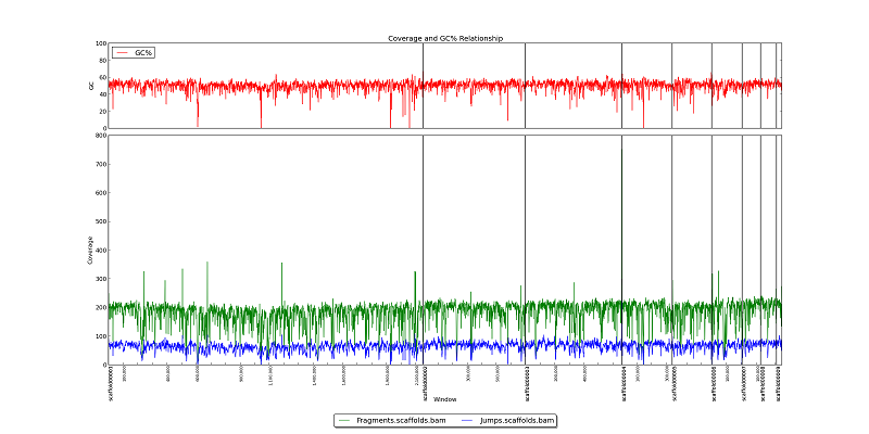
This two-part figure displays GC content, fragment read coverage, and jump read coverage across the genome as represented by the x-axis. Black vertical lines represent scaffold breaks, and tick-marks represent 100KB intervals. The red line in the upper box shows variation in GC content. Green and blue lines in the bottom box represent fragment and jump read coverage, respectively. In this example, we can see that GC content for this genome is generally about 55%, with multiple short dips to 20% or lower. The assembly has 200x fragment coverage, and 75x jump coverage. Note that we can also see a drop in fragment and jump coverage in Scaffold00006 at 100KB. Locations where coverage drops to zero are likely gaps in the scaffold sequence.
Figure 2.2:Scaffold GC Coverage Histogram (generate_bam_plots.py)
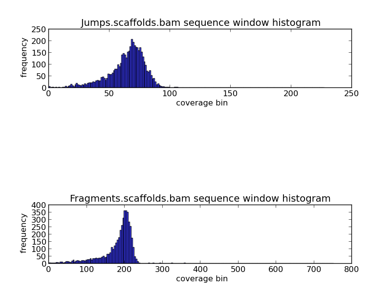
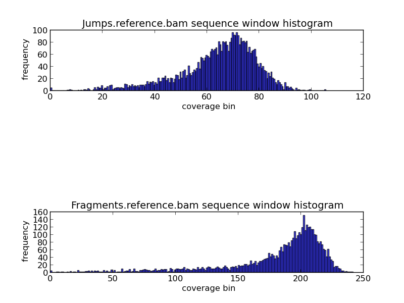
The top and bottom histograms provide information on jump and fragment coverage in the genome. Since each base can not be presented in a histogram, bins of coverage are used. The y-axis indicates the frequency of the bins, and the x-axis the coverage. For example, in the fragments histogram, we can see that the most frequent coverage in the genome is 200x coverage.
Table 2.3: Simple BAM Stats(get_simple_bam_stats.py)
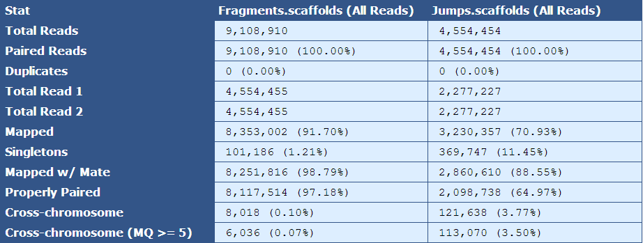
The module that creates this table generates a column for each library type in the assembly. The table below describes the contents of the table:
[table delimiter=”|”]Descriptor| Description
Total Reads| The number of reads in the assembly for each library type
Paired Reads| The number of paired reads for each library type
Duplicates| The number of duplicate reads for each library type
Total Read 1| The total number of forward reads for each library type
Total Read 2| The total number of reverse reads for each library type
Mapped| The number and percentage of reads mapping to the reference
Singletons|The number and percentage of reads in which only one mate of a read pair is present in the assembly
Mapped w/ Mate| The number and percentage of mapped reads of which the mated read is also present in the assembly
Properly Paired| The number and percentage of mated reads that are properly oriented with respect to each other and are the expected distance from each other based on insert size information
Cross-chromosome| The number and percentage of paired reads in which mates assembled in different chromosomes
Cross-chromosome (MQ >= 5)| The number and percentage of paired reads in which one mate maps to another chromosome with a mapping quality greater than or equal to 5
[/table]
Table 2.4: Sequence Coverage Stats (get_bam_coverage_stats.py)

The module that creates this table generates a column for each library type in the assembly. The table below describes the contents of the table:
[table delimiter=”|”]Descriptor| Description
Average Cvg| The mean sequence coverage across the assembly
Cvg Std Dev| The deviation in sequence coverage from the mean for the majority of reads in the assembly.
Median Cvg| The median sequence depth across the assembly
Cvg Mode| The most frequent sequence coverage level in the assembly
[/table]
Table 2.5: Physical Coverage Stats (get_bam_coverage_stats.py)

The module that creates this table generates a column for each library type in the assembly. The table below describes the contents of the Physical Coverage Stats table:
[table delimiter=”|”]Descriptor| Description
Average Cvg| The mean physical coverage across the assembly
Cvg Std Dev| The deviation in physical coverage from the mean for the majority of reads in the assembly.
Median Cvg| The median physical coverage across the assembly
Cvg Mode| The most frequent physical coverage level in the assembly
[/table]
Table 2.6: Insert Size Stats (plot_insert_size.py)
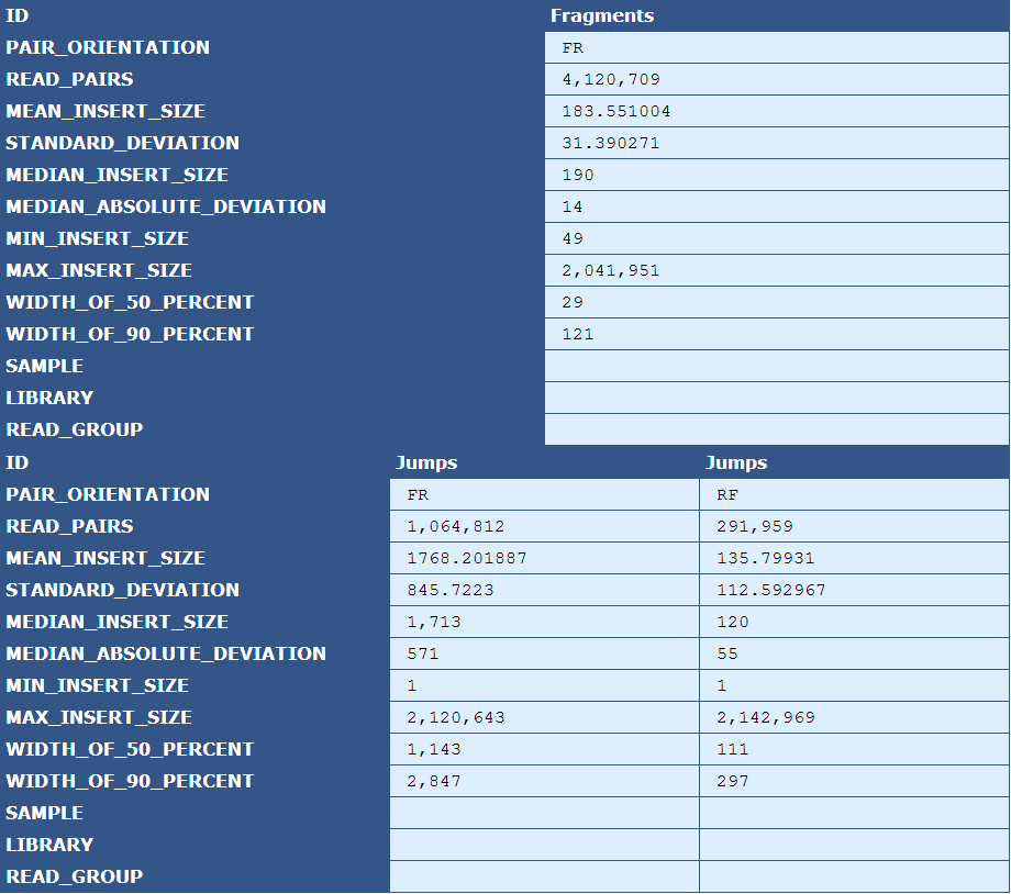
The table presents insert size statistics for fragment (top half) and jump (bottom half) reads. This example genome has two jump libraries, hence two columns of insert size data.
[table delimiter=”|”]Descriptor| Description
Pair Orientation| The orientation of the left and right reads of a pair with respect to each other(F=Forward, R=Reverse)
Read Pairs| The number of read pairs in the genome assembly
Mean Insert Size| The average insert size for the read pair
Median Absolute Deviation| A measure of the magnitude of dispersion of the insert sizes
Min Insert Size| The smallest insert size in the pool of read pairs
Max Insert Size| The largest insert size in the pool of read pairs
Width of 50 Percent| The “width” of the bins, centered around the median, that encompass 50% of all read pairs
With of 90 Percent| The “width” of the bins, centered around the median, that encompass 90% of all read pairs
Sample| The sample ID as specified by the BAM header
Library|The library ID as specified by the BAM header
Read Group| The read group as specified by the BAM header
[/table]
Figure 2.7: Scaffold Insert Size (plot_insert_size.py)

This plot shows a histogram of jump read insert sizes with an associated box plot. The box plot (using the histogram x-axis) presents several insert size metrics: minimum, first quartile, second quartile, median, third quartile, maximum, and outliers. The minimum insert size in this example is 1, and the first quartile, represented by the left-most dashed line, is the first quartile (25th percentile). The box represents the second quartile (from ~1250bp to ~2300bp), all reads between the 25th and 75th percentile (third quartile). The line bisecting the box is the median (1713bp). The horizontal dashed line to the right of the box represents all insert sizes above the 75th percentile. The vertical dash, or ‘upper fence’, represents the maximum value for the insert size, and the plus signs beyond the fence are outliers.
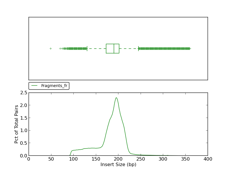
The insert size histogram presents the same data as the jump insert size histogram but for fragment reads. Note that in addition to an upper fence, the lower fence is displayed at approximately 130bp.
Figure 2.8: Coverage Anomalies Scatter Plot (IdentifyCoverageAnomalies.py)
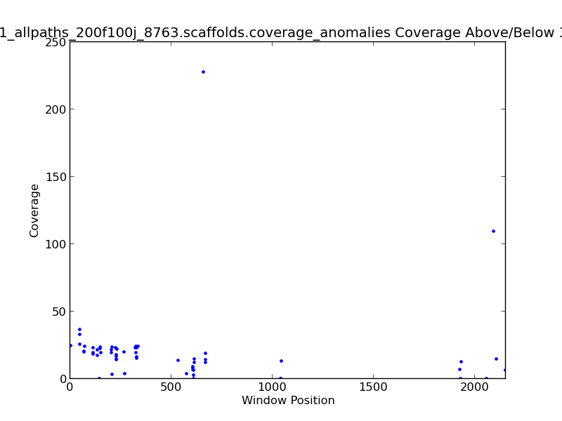
The Coverage Anomalies Scatter Plot shows the points along the genome where coverage is greater than three standard deviations from the norm. For example, this plot shows positions of high coverage at approximately 600 KB and 2.1 MB(~120x coverage).
Figure 2.9: Scaffold Coverage Anomalies Cluster Length (IdentifyCoverageAnomalies.py)
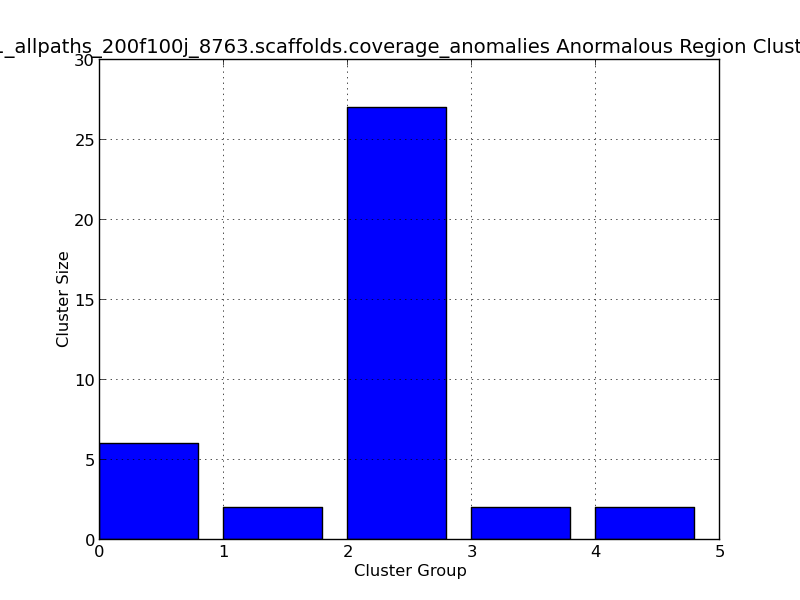
This bar graph represents clusters of regions with anomalous coverage. In this example, four anomalous clusters are represented, with the largest cluster group (#2) containing 27 positions with anomalous coverage.
Figure 2.10: Scaffold Coverage Anomalies Change in Coverage Scatter Plot (IdentifyCoverageAnomalies.py)
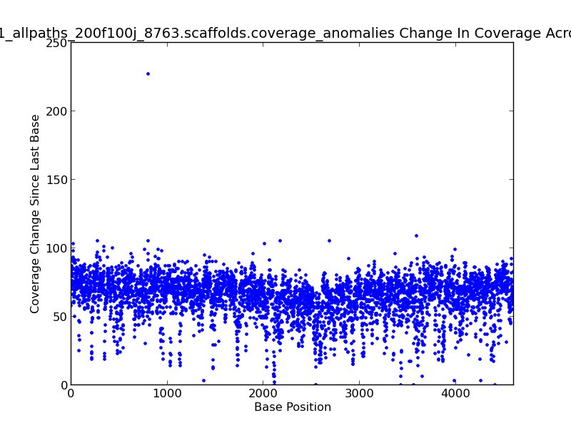
This scatter plot represents change in coverage from one base position to the next across the genome. For example, there is an approximately 235x change in coverage near 800 KB in this genome, as shown by the dot in the upper left quadrant of the plot.
Figure 2.11: Scaffold Coverage Anomalies Change in Coverage Histogram (IdentifyCoverageAnomalies.py)
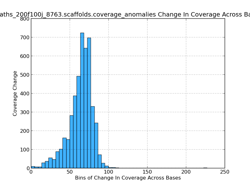 This histogram gives the analyst an idea of which coverage levels are most prevalent in the genome. Since a base-by-base analysis is not feasible sequence windows, or bins, are used. In this figure, for example, their are over 700 sequence windows in which the mean coverage change from one window to the next is about 65x.
3.2.3: Kmer Analysis
Table 3.1: Kmer Copy Number (kmer_copy_number.py)
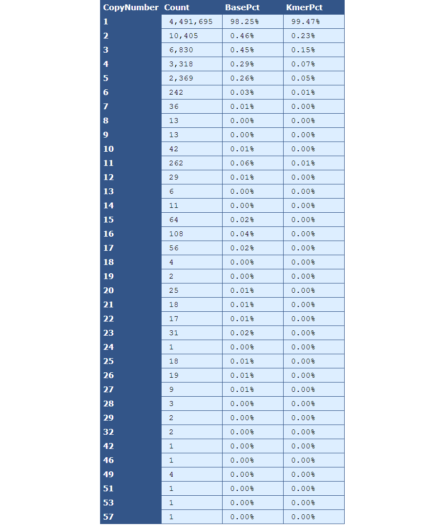
This table presents the frequency of Kmer copy numbers, with the left-most column serving as the header and each row containing frequency data for the copy number indicated by the header.
[table delimiter=”|”]Descriptor| Description
Count| The total number of Kmers for the given copy number.
BasePct| The percentage of bases from the genome that have the given copy number.
KmerPct| The percentage of Kmers that have the given copy number.
[/table]
3.2.4: Gap End Analysis
Table 4.1: Gap End Analysis Table (analyze_gap_ends.py)

This table, as the header indicates, presents metrics for both captured gaps and uncaptured ends.
[table delimiter=”|”]Descriptor| Description
Number| The total number of uncaptured ends and captured gaps (uncaptured ends should always be twice the scaffold count, and captured gaps should be the number of contigs minus scaffolds)
Average Complexity| The percentage of 5-mers near gap ends that occur once in the genome
Less than 75% Complexity| The percent of gaps that are less than 75% complex.
Average GC| The percent of Gs and Cs in the gap flanking sequence
Less than 30% GC| The number of gaps composed of less than 30% Gs and Cs
Greater than 70% GC| The number of gaps composed of greater than 70% Gs and Cs
Average Copy Number| The average number of copies of the gap sequence in the genome
[/table]
Figure 4.2: CG Sizes (analyze_gap_ends.py)
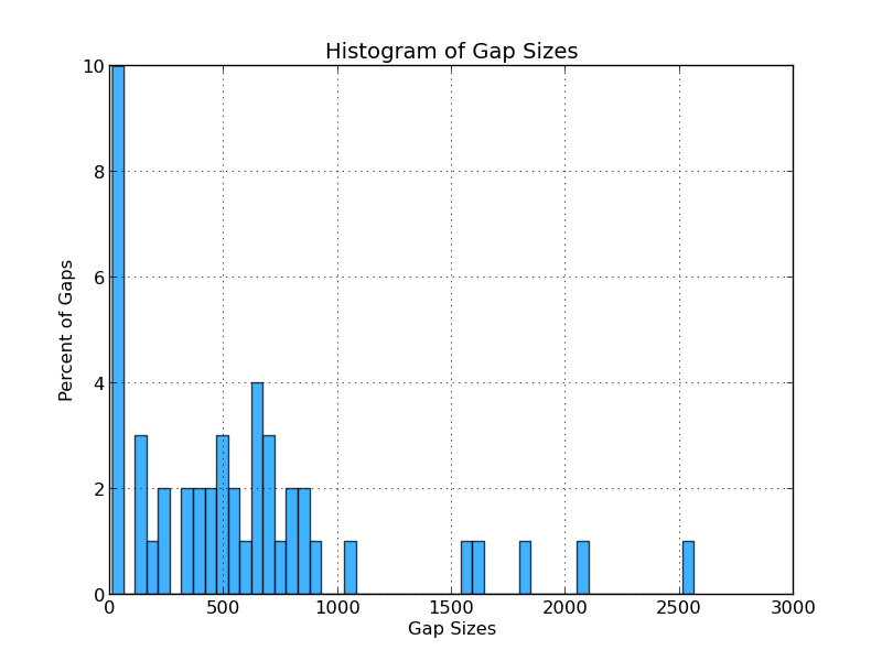
This histogram displays the percentage of gaps of various lengths. For example, 10% of the gaps in the analyzed genome are below 50 bases wide, and 4% are between 600 and 650 bases wide.
Figure 4.3: CG Complexity (analyze_gap_ends.py)
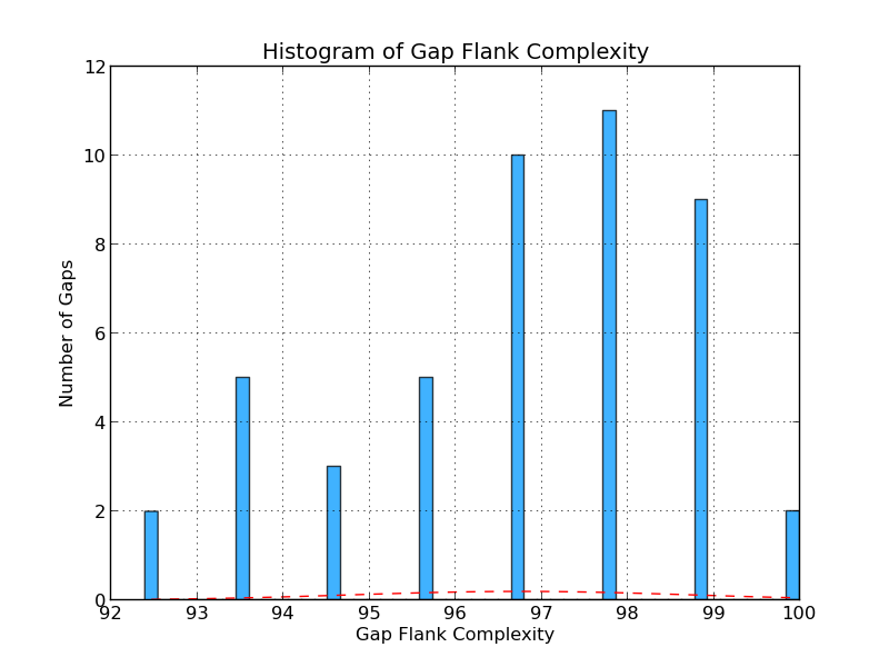
The gap flank complexity graph gives an indication of repeat content in the sequence flanking the gaps in the analyzed genome. It is calculated by examining all 5-mers in a gap’s flanking sequence (fifty bases on each side) and assessing the percentage of 5-mers that occur only once. In this example, eleven gaps have a 5-mer composition in which 98% of 5-mers occur only once.
Figure 4.4: CG Copy Number (analyze_gap_ends.py)
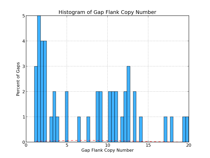 The graph presents the range of copy numbers for sequence flanking gaps as a percentage of all gaps. For example, the figure above shows that 2% of all gap flank sequences have a copy number of five.
Figure 4.5: CG GC (analyze_gap_ends.py)
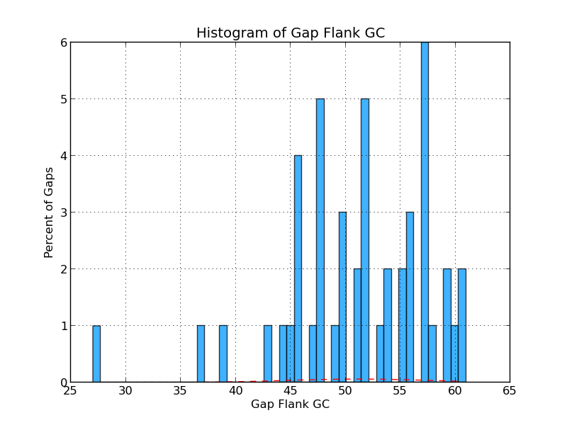
This histogram shows the frequency (in percent) of Gs and Cs across a range of GC percentages for captured gap flanking sequences. For example, 1% of the gaps have flanking sequence with 60% GC content in the figure above.
Figure 4.6: UE Distinctness (analyze_gap_ends.py)
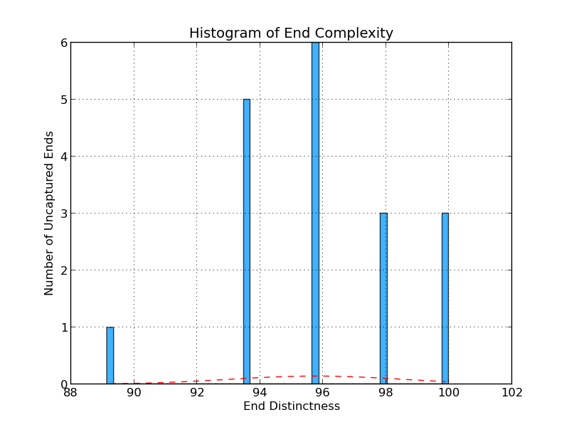
The uncaptured end flank complexity graph gives an indication of repeat content in the sequence at the end of a scaffold in the analyzed genome. It is calculated by examining all 5-mers in the end sequence (fifty bases) and assessing the percentage of 5-mers that occur only once. In this example, six gaps have a 5-mer composition in which 96% of 5-mers occur only once.
Figure 4.7: UE Copy Number (analyze_gap_ends.py)
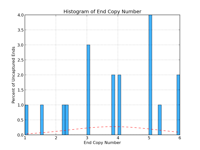
Like Figure 4.3, this graph displays sequence copy number, but in this case as a percentage of uncaptured ends. In this example, 4% of the uncaptured ends have sequence with five copies within the genome.
Figure 4.8: UE GC (analyze_gap_ends.py)
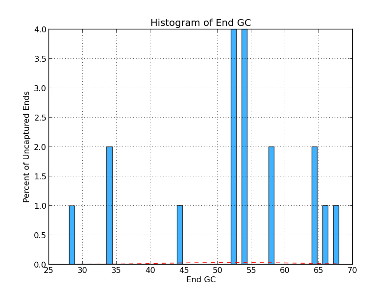 This histogram shows the frequency (in percent) of Gs and Cs across a range of GC percentages for uncaptured ends. For example, 2% of the gaps have uncaptured end sequence with 34% GC content in the figure above.
3.2.5: Reference Analysis
Figure 5.1: Alignment to Reference (run_nucmer.py)
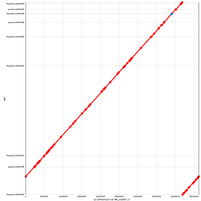
This dotplot presents a 1-to-1 alignment between the assembled genome and the reference sequence, with reference and coordinates drawn on the x-axis and scaffolds and their IDs on the y-axis. Red lines and dots represent sequence that aligns in the same sense as the reference, while blue lines (none shown here) and dots represent sequence that is complemented with respect to the reference. Note that the scaffolds marked with an asterisk are actually complemented in the assembly FASTA with respect to the reference, but are drawn in the same sense to show the actual order and orientation of the genome.
Table 5.2: Scaffold Accuracy (run_scaffold_accuracy.py)
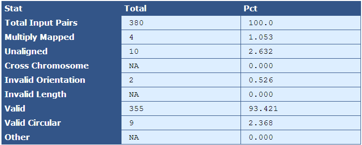
This table provides various statistics relevant to how accurately the genome assembled. Note that this actual mate pairs from the libraries are not used, but rather ‘pairoids’ are generated from the reference sequence (sequences with a fixed number of bases between them in the reference sequence designate a pairoid) and then mapped to the assembly FASTA, and various statistics are collected to give a general indication of how well the genome assembled with respect to the reference. Raw numbers and percentages are provided in the second and third columns.
| Descriptor| Description |
|---|
| Total Input Pairs| The number of pairoids sampled. |
| Multiply Mapped| The number and percent of pairoids from the sample that map to more than one location in the genome's reference sequence |
| Unaligned| The number and percent of pairoids that do not map to the genome's reference sequence |
| Cross Chromosome| The number and percent of pairoids in which pairs map to two different chromosomes |
| Invalid Orientation| The number and percent of pairoids in which the orientation is invalid. For most libraries, valid orientation is when the left read has a forward orientation, and the right read has a reverse orientation |
| Invalid Length| The number and percent of pairoids separated by more or less than the allowable number of bases apart |
| Valid | The number and percent of pairoids with valid orientation and length |
| Valid Circular | The number and percent of pairoids that create circularity from one end of the scaffold to the other. |
Note that the definition of ‘cross chromosome’ depends on the reference used for the assembly. Specifically, when the reads of a pairoid map to two different elements (chromosomes, plasmids scaffolds) in the FASTA file, they will be labeled as cross chromosome. In a finished reference with multiple chromosomes, the meaning is as expected. If a finished reference contains chromosomes and plasmid, it could mean that one read in a pairoid maps to a plasmid, and the other to a chromosome, and in an unfinished reference, it could mean that one read in a pairoid maps to a different scaffold that may or may not be part of the same chromosome.
Table 5.3: Kmer Coverage (kmer_coverage.py)

This table provides more detailed information on the kmer coverage across the analyzed genome by providing the total number bases in the kmers, bases covered in the reference, and percent of reference covered for multiple categories.
| Descriptor| Description |
|---|
| Covered | The total bases in the kmers, the total bases that align to the reference, and percentage of total that align to the reference |
| DistinctCovered | The distinct bases in the kmers with copy number of one, the total bases that align to the reference, and percentage of total that align to the reference |
| OverCovered | The bases in the kmers with copy number greater than one, the total bases that align to the reference, and percentage of total that align to the reference |
| Novel | The bases in kmers that are novel and the percentage of the genome that these novel bases composes |
| NovelDistinct | The bases in kmers with a copy number of one that are novel and the percentage of the genome that these novel bases composes |
Figure 5.4: Coverage and GC Line Plot
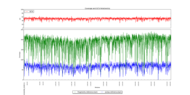
Like figure 2.1, this plot displays GC Content, fragment read coverage, and jump read coverage, but in this plot, the x-axis represents the reference genome and not the actual assembly.
Figure 5.5: GC Coverage Histogram (generate_bam_plots.py)
The histograms shown above display the frequency of various coverage levels when jump and fragment reads are aligned to the reference genome. In this example, we can see that the most frequent coverage is about 70x to 75x in jump reads, and about 210x to 220x in fragment reads.
Table 5.6: Reference Simple BAM Stats Table (get_simple_bam_stats.py)
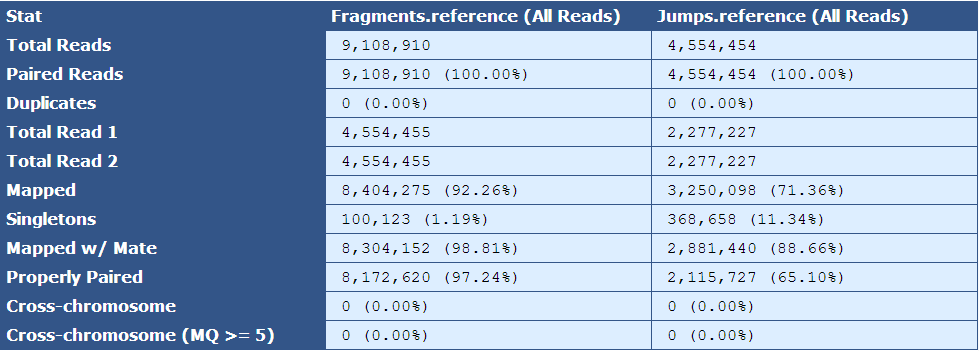
Like Table 2.1, this table presents simple BAM stats, but with respect to the reads as they align to the reference sequence.
| Descriptor| Description | |
|---|---|
| Total Reads| The number of reads in the assembly for each library type | |
| Paired Reads| The number of paired reads for each library type | |
| Duplicates| The number of duplicate reads for each library type | |
| Total Read 1| The total number of forward reads for each library type | |
| Total Read 2| The total number of reverse reads for each library type | |
| Mapped| The number and percentage of reads mapping to the reference | |
| Singletons|The number and percentage of reads in which only one mate of a read pair is present in the assembly | |
| Mapped w/ Mate| The number and percentage of mapped reads of which the mated read is also present in the assembly | |
| Properly Paired| The number and percentage of mated reads that are properly oriented with respect to each other and are the expected distance from each other based on insert size information | |
| Cross-chromosome| The number and percentage of paired reads in which mates assembled in different chromosomes | |
| Cross-chromosome (MQ | gt;= 5)| The number and percentage of paired reads with mapping quality greater than or equal to 5 in which mates assembled in different chromosomes |
Table 5.7: Reference Sequence Coverage Stat (get_bam_coverage_stats.py)

This table provides statistics on how well the fragment and jump read sequences cover the reference sequence.
| Descriptor | Description |
|---|---|
| Average Cvg | The mean sequence coverage across the reference |
| Cvg Std Dev | The deviation in sequence coverage from the mean for the majority of reads in the reference. |
| Median Cvg | The median sequence depth across the reference |
| Cvg Mode | The most frequent sequence coverage level in the reference |
Table 5.8: Physical Coverage Stats (get_bam_coverage_stats.py)
This table provides statistics on how well the fragment and jump reads physically cover the reference sequence.
| Descriptor | Description |
|---|---|
| Average Cvg | The mean sequence coverage across the reference |
| Cvg Std Dev | The deviation in sequence coverage from the mean for the majority of reads in the reference. |
| Median Cvg | The median sequence depth across the reference |
| Cvg Mode | The most frequent sequence coverage level in the reference |
Figure 5.9: Insert Size (plot_insert_size.py)
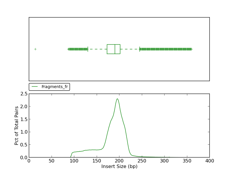
This insert size histogram presents the same data as the jump insert size histograms shown in figures 5.8 and 2.5, but for fragment reads. Like figure 2.5, this example shows a lower fence (at ~140bp) as well as an upper fence (at ~ 250bp).
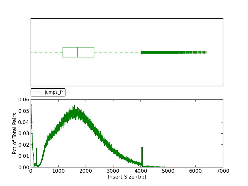
This plot shows a histogram of jump read insert sizes with an associated box plot. The box plot (using the histogram x-axis) presents several insert size metrics: minimum, first quartile, second quartile, median, third quartile, maximum, and outliers. The minimum insert size in this example is 1, and the first quartile, represented by the left-most dashed line, is the first quartile (25th percentile). The box represents the second quartile (from ~1250bp to ~2300bp), all reads between the 25th and 75th percentile (third quartile). The line bisecting the box is the median (1730 bp). The horizontal dashed line to the right of the box represents all insert sizes above the 75th percentile. The vertical dash, or ‘upper fence’, represents the maximum value for the insert size, and the plus signs beyond the fence are outliers.
Table 5.10: Insert Size Stats (plot_insert_size.py)
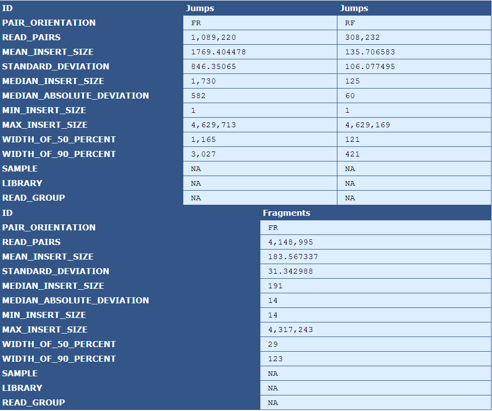
The table presents insert size statistics for fragment (top half) and jump (bottom half) reads. This example genome has two jump libraries, hence two columns of insert size data.
| Descriptor | Description |
|---|---|
| Pair Orientation | The orientation of the left and right reads of a pair with respect to each other(F=Forward, R=Reverse) |
| Read Pairs | The number of read pairs in the genome assembly |
| Mean Insert Size | The average insert size for the read pair |
| Median Absolute Deviation | A measure of the magnitude of dispersion of the insert sizes |
| Min Insert Size | The smallest insert size in the pool of read pairs |
| Max Insert Size | The largest insert size in the pool of read pairs |
| Width of 50 Percent | The "width" of the bins, centered around the median, that encompass 50% of all read pairs |
| With of 90 Percent | The "width" of the bins, centered around the median, that encompass 90% of all read pairs |
| Sample | The sample name, if available in the BAM file header |
| Library | The library name, if available in the BAM file header |
| Read Group | The read group name, if available in the BAM file header |
Figure 5.11: Comparison To Reference
The Comparison to Reference Table shows a base-count comparison of shared and novel sequence between the assembled genome and the reference genome. In this example, there are 39 sequence regions that are present in the reference but not the assembly, and 44 sequences present in the assembly but not the reference.
| Descriptor | Description |
|---|---|
| Fasta File ID | The names of the fasta files being compared |
| Total Length (bp) | The total length of the reference and assembly sequences |
| Total Novel Regions | The total number of novel regions in the reference and assembly sequences |
| Total Novel Bases (bp) | The total number of bases among all novel regions |
| Average Novel Region Size (bp) | The average size of novel regions in each sequence |
| Largest Novel Region Size (bp) | The largest novel region in each sequence |
| N50 Novel Region Size (bp) | The N50 size of the novel regions in each sequence |
| Pct Covered | The percent of sequence covered in one sequence by the comparison sequence |
| Pct Identity | The percent identity, or sequence similarity, of the two sequences to each other. |
Figure 5.12: Coverage Anomalies Scatter Plot (IdentifyCoverageAnomalies.py)
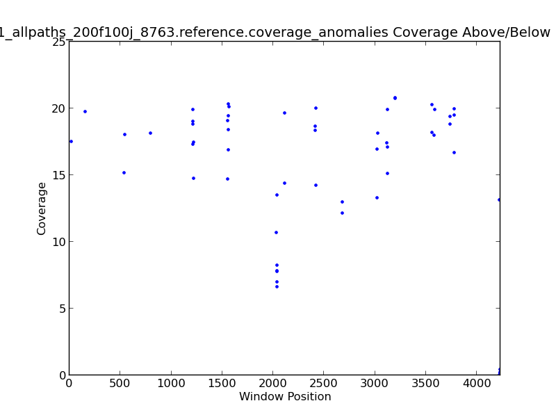
The Coverage Anomalies Scatter Plot shows the points along the genome where coverage is greater than two standard deviations from the norm.
Figure 5.13: Coverage Anomalies Bar Plot (IdentifyCoverageAnomalies.py)
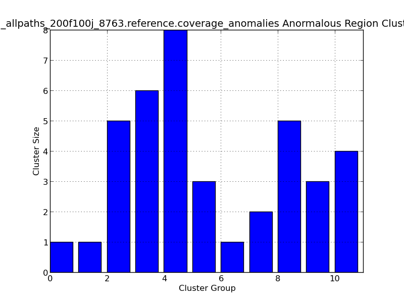
This bar graph represents cluster of regions with anomalous coverage. In this example, ten anomalous clusters are represented, with the largest cluster group (#4) containing 8 positions with anomalous coverage.
Figure 5.14: Coverage Change Across Bases Scatter Plot (IdentifyCoverageAnomalies.py)
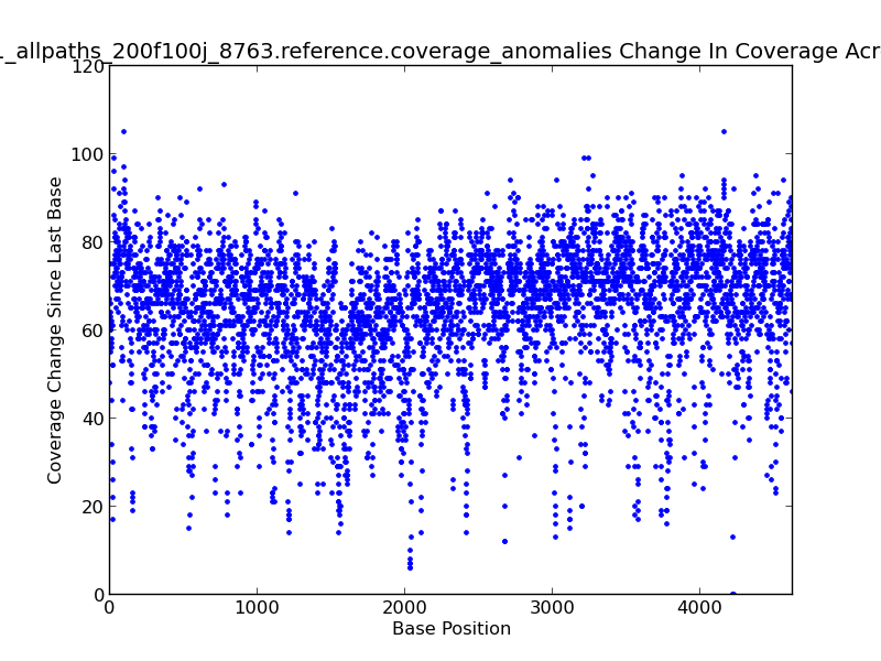
This scatter plot represents change in coverage from one base position to the next across the genome. For example, there is an approximately 105x change in coverage near the beginning of this genome, as shown by upper-left-most dot in the figure.
Figure 5.15: Coverage Change Across Bases Histogram (IdentifyCoverageAnomalies.py)
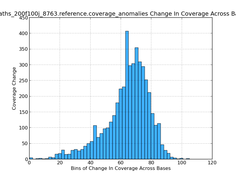 This histogram shows the frequency of coverage changes and gives an indication of how variable the coverage is in the genome. In this exmaple, most coverage changes are near ~70x.
3.2.6: Blast Analysis
Figure 6.1: Blast Bubbles (blast_bubbles.py)
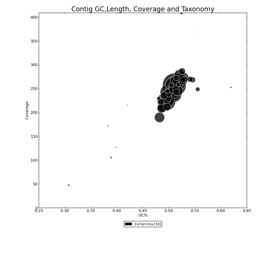
This bubble plot shows four pieces of information to display the taxonomic makeup of the genome assembly. Coverage depth is represented on the y-axis, and percent GC on the x-axis.The color key beneath x-axis indicates the different organisms in the assembly based on Blast results, and the number inside brackets indicates how many contigs match that genus. Contigs are drawn as bubbles at the intersection of their coverage depth and percent GC values. The size of the bubble indicates the length of the contig, and the color its taxonomy. In this example, we see that there is a small contig with just under 50x coverage and ~31% GC content that aligns to Escherichia, and that most of the large contigs in this assembly range from 200x to 300x coverage, 47% to 57% GC, and that all contigs align to Escherichia genus.
Figure 6.2: Blast Heat Map (blast_map.py)
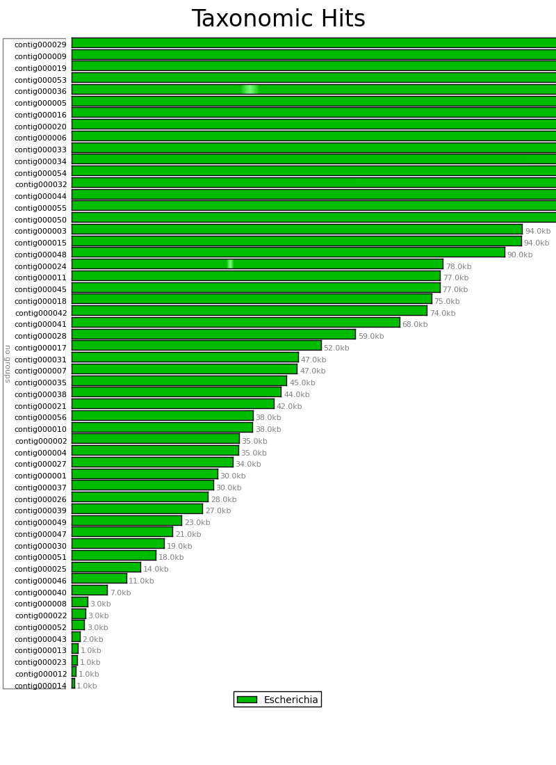
The Blast Heat Map indicates the degree to which the sequence in the contigs of the assembly match the reference sequence, with darker shading indicating a strong match, and lighter shading indicating a weak match. In this example we can see that all the contigs strongly match Escherichia, though contigs 36 and 24 have each have a small region with weaker matches.
Table 6.3: Blast Taxonomy Details (get_blast_hit_taxonomy.py)
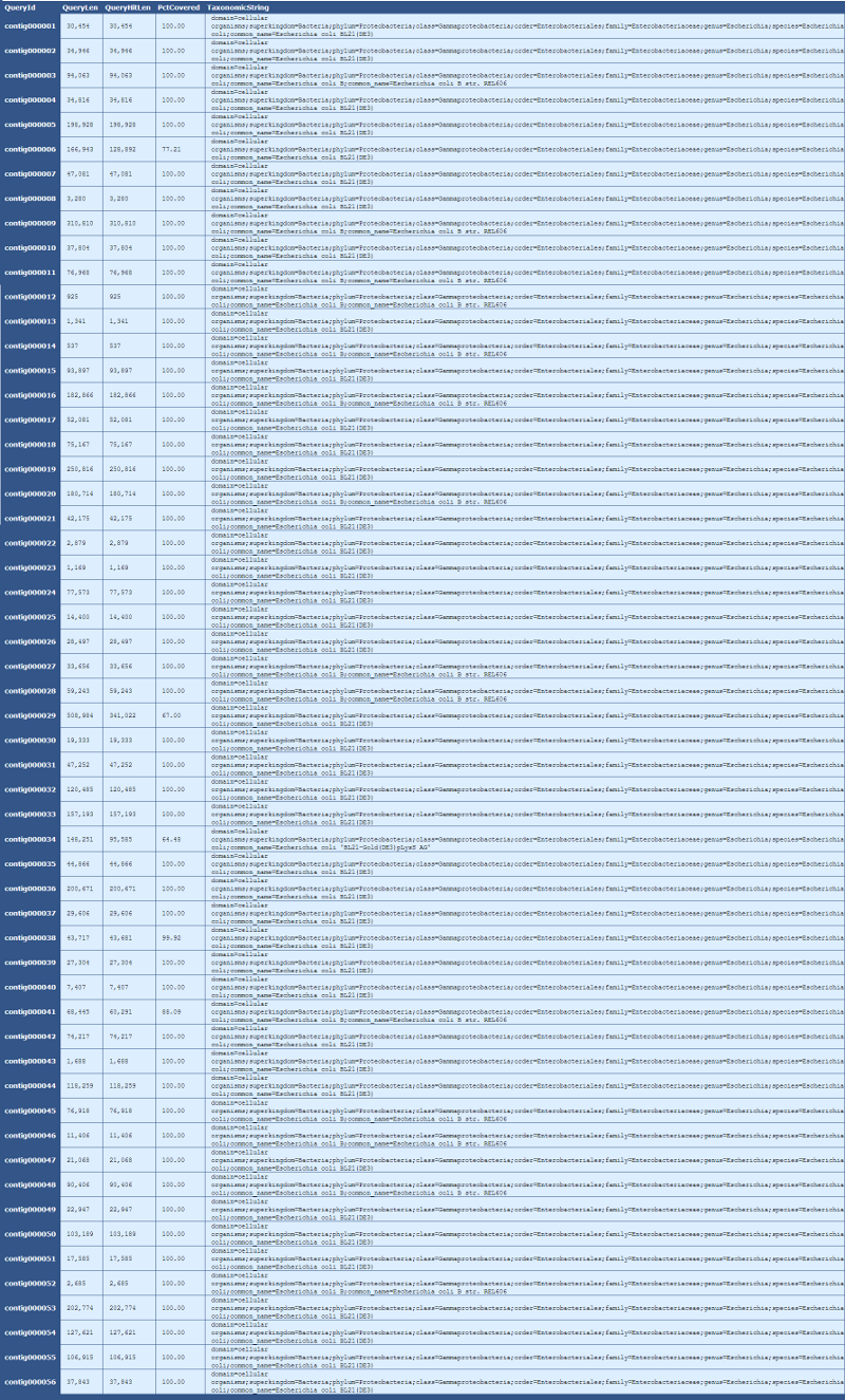
This table provides details taxonomic information for each contig in the genome, as described below:
[table delimiter=”|”]
Descriptor| Description
QueryID | The contig name
QueryLen | The length in bases of the contig
QueryHitLen | The length in based of the matched alignment
PctCovered | The percent of the contig matched by the aligned sequence
TaxonomicString | The full taxonomic information, from domain to species, of the aligned sequence
[/table]
In this table, we can see that 77%, or 128 of 166kb, of contig000006 aligns to Escherichia coli BL21(DE3).
3.2.7: rRNA Details
Table 7.1: rRNA Analysis Details (analyze_rna_hits.py)
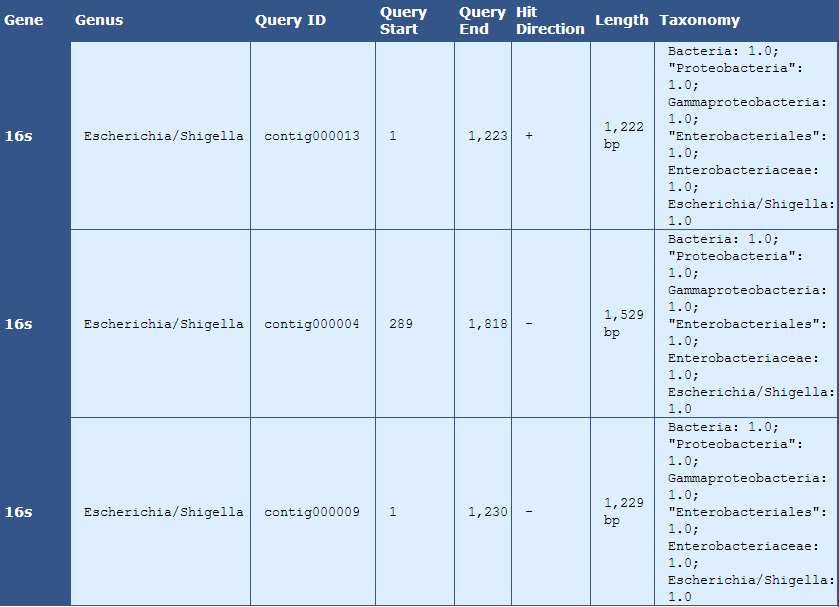
This table displays 16s rRNA hits
[table delimiter=”|”]
Descriptor| Description
Gene | The aligned gene
Genus | The genus of the organism of the aligned gene
Query ID | The contig containing the aligned gene sequence
Query Start | The start position of the aligned gene sequence
Query End | The end position of the aligned gene sequence
Hit Direction | The direction of the alignment with regards to the contig sequence
Length | The length in bases of the sequence alignment
Taxonomy | The taxomomic information of the aligned sequence
[/table]
3.2.8: Assembly Details
Table 8.1: Contig Details (make_detailed_assembly_table.py )
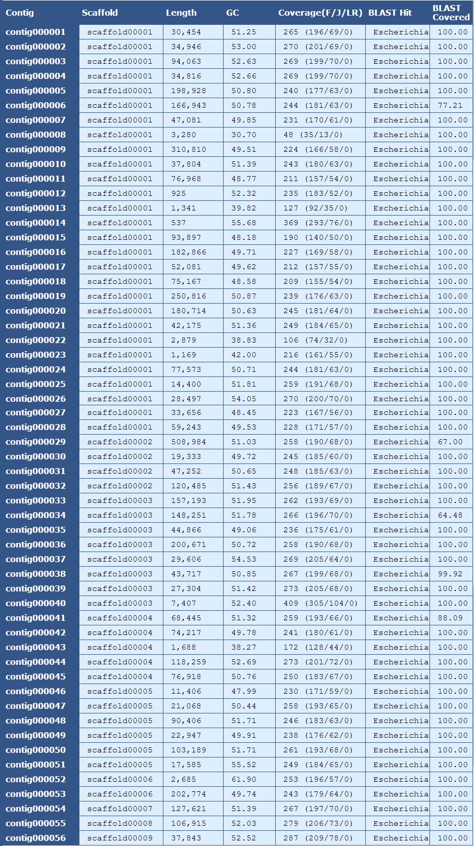
The table above provides summary details for each contig in the assembly as listed below:
[table delimiter=”|”]
Descriptor| Description
Contig| The name of the contig
Scaffold| The scaffold that contains the contig
Length| The length of the contig
GC| The average GC content of the contig
Coverage (F/J/L)| The mean coverage for the contig. A breakdown of fragment(F), jump(J), and long read(LR) coverage is shown in the parentheses
BLAST Hit| The genus of the top blast hit for the contig
BLAST Covered| The percent of the contig’s sequence aligning to the top blast hit
[/table]
Table 8.2: Scaffold Details (make_detailed_assembly_table.py )

The Scaffold Details Table provides information on the number of contigs, length, %GC content, coverage, BLAST alignment, and circularity for each scaffold in the assembly.
[table delimiter=”|”]
Descriptor| Description
Scaffold| The name of the scaffold
Num Contigs| The number of contigs contained within the scaffold
Length| The length of the scaffold
GC| The average GC content of the scaffold
Coverage (F/J/L)| The mean coverage for the scaffold. A breakdown of fragment(F), jump(J), and long read(L) coverage is shown in the parentheses
BLAST Hit| The genus of the top blast hit for the scaffold
BLAST Covered| The percent of the scaffold’s sequence aligning to the top blast hit
Circular| The number of circular reads in the scaffold
[/table]


